Page
Prerequisites and step-by-step guide

Prerequisites
Step-by-step guide
1. Launch a Jupyter notebook with TensorFlow server image
To get started, we'll establish a new Data Science project within OpenShift AI that leverages a pre-configured TensorFlow image. This image provides a ready-to-use environment for building and training your machine learning models. Before proceeding, make sure you have the Red Hat Developer Sandbox set up. If not, check here for more information.
Creating a New Workbench in OpenShift AI
Launch the Red Hat Developer Sandbox by clicking here, then select the "Red Hat OpenShift AI" tile, as shown in Figure 1 below.

Login to OpenShift AI and navigate to the "Data Science project" on the left menu. You will find an already created data science project associated with your username, similar to what is shown in Figure 2 below.
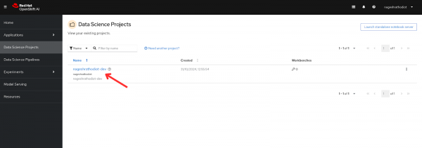
When you click on the project which is listed, you will land on the Overview page of a Data Science project similar to what is shown in Figure 3 below.
1.1 Create a Workbench
1.2 Configure the Workbench
- Provide a descriptive name for your workbench.
- Under "Notebook image" select "TensorFlow" and keep the version set to "Recommended".
- In the "Deployment size" section, choose "Medium" for the container size.
- Change the "Cluster storage" setting to 10Gi.
- After all details are filled in, you will get a similar form as shown in Figure 4 below.
Click on "Create workbench" to initiate the creation process and launch your new workbench environment.
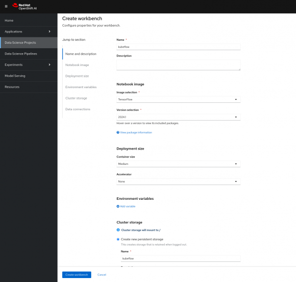
Figure 4: Workbench configuration form.
1.3 Verify Workbench Status and access Jupyter Notebook
- After clicking on "Create workbench", monitor the workbench status. It should eventually transition to "Running", indicating the successful creation of the workbench. See Figure 5 below.
Click on the "Open ↗" button located next to the status.
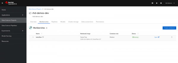
Figure 5: Workbench is in Running status. You will then land on the following Login page to authenticate yourself, click on the "DevSandbox" button, as shown in Figure 6 below.
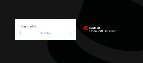
Figure 6: Login in Openshift Developer Sandbox. You might encounter a permission prompt. Select the option "Allow selected permissions" to grant the necessary access, similar to as shown in Figure 7 below.
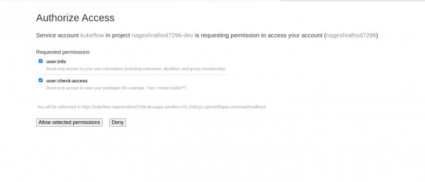
Figure 7: Authorizing permissions. After allowing permissions, you will be redirected to the JupyterLab launcher and select "Python" similar to Figure 8. The Jupyter Notebook environment will come pre-configured with TensorFlow and its dependencies.
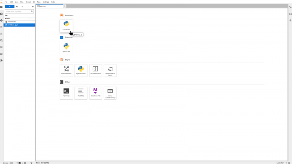
Figure 8: Jupyter launcher page. You will land on a blank Jupyter notebook as shown in Figure 9 below.
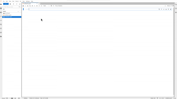
Figure 9: Accessing Jupyter notebook.
In the upcoming section, you will execute Python code in the Jupyter notebook. Copy each code snippet provided below, paste it into a notebook cell, and execute it.
Alternatively, you can clone this GitHub repository that contains the complete code in a Jupyter notebook. After cloning the repository, navigate to the "openshift-ai/4_Models_inferencing" directory and open the "Fraud_detection_model_with_tensorflow.ipynb" notebook. This notebook includes all the necessary code snippets, along with detailed explanations and a discussion of the results, essential for completing this learning exercise.
The following code snippets assume that the current directory is set to "openshift-ai/4_Models_inferencing". Be sure to navigate to this directory before running the code snippets.
2. Install Python dependencies
In this exercise, we will use a sklearn model to create, train, and make predictions from the trained model. We will also handle model saving locally. Before saving, we'll save the model in pickle format and convert it to an ONNX model, as shown in the code snippets below. This approach ensures that our model is both efficient and compatible with various deployment environments.
Start by executing the following command to install the Python packages which are required by this learning exercise.
!pip install onnx onnxruntime seaborn tf2onnxExpected output:
Collecting onnxruntime
  Downloading onnxruntime-1.18.1-cp39-cp39-manylinux_2_27_x86_64.manylinux_2_28_x86_64.whl (6.8 MB)
     ━━━━━━━━━━━━━━━━━━━━━━━━━━━━━━━━━━━━━━━━ 6.8/6.8 MB 70.9 MB/s eta 0:00:00a 0:00:01
Collecting seaborn
  Downloading seaborn-0.13.2-py3-none-any.whl (294 kB)
     ━━━━━━━━━━━━━━━━━━━━━━━━━━━━━━━━━━━━━ 294.9/294.9 kB 313.6 MB/s eta 0:00:00
The imported libraries and modules facilitate various tasks in machine learning and data processing. NumPy and Pandas handle numerical and data manipulation, while Keras provides tools for building and training neural networks. Scikit-learn aids in data preprocessing and model evaluation, and tf2onnx along with onnx allows for model interoperability between frameworks. Pickle is used for object serialization, and Path simplifies file path operations.
import numpy as np
import pandas as pd
import datetime
from keras.models import Sequential
from keras.layers import Dense, Dropout, BatchNormalization, Activation
from sklearn.model_selection import train_test_split
from sklearn.preprocessing import StandardScaler
from sklearn.utils import class_weight
import tf2onnx
import onnx
import pickle
from pathlib import Path
3. Load and process the dataset
In this processes data for a fraud detection model by extracting specific features and labels from training, validation, and test datasets. It scales input features to zero mean and unit variance using StandardScaler, fitting the scaler only on the training data to avoid data leakage. The test data and scaler object are saved as artifacts (.pkl files) for future use. Additionally, it computes class weights to address dataset imbalance, giving higher importance to fraudulent transactions during model training.
# Set the input (X) and output (Y) data.
# The only output data is whether it's fraudulent. All other fields are inputs to the model.

feature_indexes = [
    1,  # distance_from_last_transaction
    2,  # ratio_to_median_purchase_price
    4,  # used_chip
    5,  # used_pin_number
    6,  # online_order
]

label_indexes = [
    7  # fraud
]

df = pd.read_csv('data/train.csv')
X_train = df.iloc[:, feature_indexes].values
y_train = df.iloc[:, label_indexes].values

df = pd.read_csv('data/validate.csv')
X_val = df.iloc[:, feature_indexes].values
y_val = df.iloc[:, label_indexes].values

df = pd.read_csv('data/test.csv')
X_test = df.iloc[:, feature_indexes].values
y_test = df.iloc[:, label_indexes].values


# Scale the data to remove mean and have unit variance. The data will be between -1 and 1, which makes it a lot easier for the model to learn than random (and potentially large) values.
# It is important to only fit the scaler to the training data, otherwise you are leaking information about the global distribution of variables (which is influenced by the test set) into the training set.

scaler = StandardScaler()

X_train = scaler.fit_transform(X_train)
X_val = scaler.transform(X_val)
X_test = scaler.transform(X_test)

Path("artifact").mkdir(parents=True, exist_ok=True)
with open("artifact/test_data.pkl", "wb") as handle:
    pickle.dump((X_test, y_test), handle)
with open("artifact/scaler.pkl", "wb") as handle:
    pickle.dump(scaler, handle)

# Since the dataset is unbalanced (it has many more non-fraud transactions than fraudulent ones), set a class weight to weight the few fraudulent transactions higher than the many non-fraud transactions.
class_weights = class_weight.compute_class_weight('balanced', classes=np.unique(y_train), y=y_train.ravel())
class_weights = {i : class_weights[i] for i in range(len(class_weights))}
No output expected here.
4. Build the model
We define a neural network using Keras with several Dense layers, Dropout layers, and Batch Normalization, configured for binary classification. It compiles the model with the Adam optimizer and binary cross-entropy loss, and then prints the model summary. Using the following model code snippet.
model = Sequential()
model.add(Dense(32, activation='relu', input_dim=len(feature_indexes)))
model.add(Dropout(0.2))
model.add(Dense(32))
model.add(BatchNormalization())
model.add(Activation('relu'))
model.add(Dropout(0.2))
model.add(Dense(32))
model.add(BatchNormalization())
model.add(Activation('relu'))
model.add(Dropout(0.2))
model.add(Dense(1, activation='sigmoid'))

model.compile(
    optimizer='adam',
    loss='binary_crossentropy',
    metrics=['accuracy']
)

model.summary()
The model summary shows a sequential neural network with various layers including Dense, Dropout, Batch Normalization, and Activation. It indicates the output shape and the number of trainable parameters for each layer, with a total of 2593 parameters.
Expected output:
Model: "sequential"

┏━━━━━━━━━━━━━━━━━━━━━━━━━━━━━━━━━┳━━━━━━━━━━━━━━━━━━━━━━━━┳━━━━━━━━━━━━━━━┓
┃ Layer (type)                    ┃ Output Shape           ┃       Param # ┃
┡━━━━━━━━━━━━━━━━━━━━━━━━━━━━━━━━━╇━━━━━━━━━━━━━━━━━━━━━━━━╇━━━━━━━━━━━━━━━┩
│ dense (Dense)                   │ (None, 32)             │           192 │
├─────────────────────────────────┼────────────────────────┼───────────────┤
│ dropout (Dropout)               │ (None, 32)             │             0 │
├─────────────────────────────────┼────────────────────────┼───────────────┤
│ dense_1 (Dense)                 │ (None, 32)             │         1,056 │
├─────────────────────────────────┼────────────────────────┼───────────────┤
│ batch_normalization             │ (None, 32)             │           128 │
│ (BatchNormalization)            │                        │               │
├─────────────────────────────────┼────────────────────────┼───────────────┤
│ activation (Activation)         │ (None, 32)             │             0 │
├─────────────────────────────────┼────────────────────────┼───────────────┤
│ dropout_1 (Dropout)             │ (None, 32)             │             0 │
├─────────────────────────────────┼────────────────────────┼───────────────┤
│ dense_2 (Dense)                 │ (None, 32)             │         1,056 │
├─────────────────────────────────┼────────────────────────┼───────────────┤
│ batch_normalization_1           │ (None, 32)             │           128 │
│ (BatchNormalization)            │                        │               │
├─────────────────────────────────┼────────────────────────┼───────────────┤
│ activation_1 (Activation)       │ (None, 32)             │             0 │
├─────────────────────────────────┼────────────────────────┼───────────────┤
│ dropout_2 (Dropout)             │ (None, 32)             │             0 │
├─────────────────────────────────┼────────────────────────┼───────────────┤
│ dense_3 (Dense)                 │ (None, 1)              │            33 │
└─────────────────────────────────┴────────────────────────┴───────────────┘

Total params: 2,593 (10.13 KB)
Trainable params: 2,465 (9.63 KB)
Non-trainable params: 128 (512.00 B)
5. Train the model
Train a machine learning model and measure the training duration. It utilizes the fit method to train the model on the specified dataset for two epochs while validating its performance on a separate validation set. Class weights are applied to address data imbalance, and training progress is logged. Finally, the total training time is calculated and reported.
# Train the model and get performance
import os
import time

start = time.time()
epochs = 2
history = model.fit(
    X_train,
    y_train,
    epochs=epochs,
    validation_data=(X_val, y_val),
    verbose=True,
    class_weight=class_weights
)
end = time.time()
print(f"Training of model is complete. Took {end-start} seconds")
We are training the model for 2 epochs, with each epoch consisting of 18750 steps.
Expected output:
Epoch 1/2
18750/18750 ━━━━━━━━━━━━━━━━━━━━ 69s 3ms/step - accuracy: 0.8942 - loss: 0.2964 - val_accuracy: 0.9506 - val_loss: 0.2139
Epoch 2/2
18750/18750 ━━━━━━━━━━━━━━━━━━━━ 65s 3ms/step - accuracy: 0.9476 - loss: 0.2355 - val_accuracy: 0.9520 - val_loss: 0.2256
Training of model is complete. Took 134.21636605262756 seconds
Training of the model is complete.
6. Save the model file
The following code snippet converts a Keras model to the ONNX format for compatibility with ModelMesh, which is a platform for managing machine learning models. Thereafter, it saves the trained model in the model directory.
import tensorflow as tf

# Wrap the model in a `tf.function`
@tf.function(input_signature=[tf.TensorSpec([None, X_train.shape[1]], tf.float32, name='dense_input')])
def model_fn(x):
    return model(x)

# Convert the Keras model to ONNX
model_proto, _ = tf2onnx.convert.from_function(
    model_fn,
    input_signature=[tf.TensorSpec([None, X_train.shape[1]], tf.float32, name='dense_input')]
)

# Save the model as ONNX for easy use of ModelMesh
os.makedirs("models/fraud/1", exist_ok=True)
onnx.save(model_proto, "models/fraud/1/model.onnx")
7. Confirm the model file was created successfully
List the available models in the "model" directory using the following command. The output should include the model's name, size, and date.
! ls -alRh ./models/Expected output:
./models/:
total 12K
drwxr-sr-x.  3 1004770000 1004770000 4.0K Jul  1 14:43 .
drwxrwsr-x. 13 1004770000 1004770000 4.0K Jul  1 15:52 ..
drwxr-sr-x.  3 1004770000 1004770000 4.0K Jul  1 14:43 fraud

./models/fraud:
total 12K
drwxr-sr-x. 3 1004770000 1004770000 4.0K Jul  1 14:43 .
drwxr-sr-x. 3 1004770000 1004770000 4.0K Jul  1 14:43 ..
drwxr-sr-x. 2 1004770000 1004770000 4.0K Jul  1 14:43 1

./models/fraud/1:
total 24K
drwxr-sr-x. 2 1004770000 1004770000 4.0K Jul  1 14:43 .
drwxr-sr-x. 3 1004770000 1004770000 4.0K Jul  1 14:43 ..
-rw-r--r--. 1 1004770000 1004770000  13K Jul  1 15:53 model.onnx
8. Test the model
Importing dependency libraries about the sklearn so we can handle the "pickle" models, matplotlib and seaborn to print the diagrams and many more.
from sklearn.metrics import confusion_matrix, ConfusionMatrixDisplay
import numpy as np
import pickle
import onnxruntime as rt
This loads previously saved objects using pickle. It reads the scalar object from 'artifact/scaler.pkl' and the test data (X_test, y_test) from 'artifact/test_data.pkl'. This is useful for reusing the scalar to transform data or evaluate the model on previously saved test data without retraining the model.
with open('artifact/scaler.pkl', 'rb') as handle:
    scaler = pickle.load(handle)
with open('artifact/test_data.pkl', 'rb') as handle:
    (X_test, y_test) = pickle.load(handle)
Create an ONNX inference runtime session and predict values for all test inputs:
sess = rt.InferenceSession("models/fraud/1/model.onnx", providers=rt.get_available_providers())
input_name = sess.get_inputs()[0].name
output_name = sess.get_outputs()[0].name
y_pred_temp = sess.run([output_name], {input_name: X_test.astype(np.float32)})
y_pred_temp = np.asarray(np.squeeze(y_pred_temp[0]))
threshold = 0.95
y_pred = np.where(y_pred_temp > threshold, 1, 0)
The following code snippet calculates the accuracy of predictions by comparing y_test (true labels) with y_pred (predicted labels) and prints the accuracy score. It then generates a confusion matrix using confusion_matrix from Scikit-learn, visualizes it with a heatmap using Seaborn, and displays it using Matplotlib. This helps in evaluating the model’s performance by showing the number of true positives, true negatives, false positives, and false negatives.
from sklearn.metrics import precision_score, recall_score, confusion_matrix, ConfusionMatrixDisplay
import numpy as np

y_test_arr = y_test.squeeze()
correct = np.equal(y_pred, y_test_arr).sum().item()
acc = (correct / len(y_pred)) * 100
precision = precision_score(y_test_arr, np.round(y_pred))
recall = recall_score(y_test_arr, np.round(y_pred))

print(f"Eval Metrics: \n Accuracy: {acc:>0.1f}%, "
      f"Precision: {precision:.4f}, Recall: {recall:.4f} \n")

c_matrix = confusion_matrix(y_test_arr, y_pred)
ConfusionMatrixDisplay(c_matrix).plot()
The confusion matrix heatmap reveals that the model achieves an accuracy of 97.21%, indicating strong overall performance. It correctly classifies a significant number of transactions, with 181,306 true negatives and 13,107 true positives. The model exhibits high precision, effectively identifying fraudulent transactions with minimal false positives (1,193). However, the recall is lower, with 4,394 false negatives, suggesting that some fraudulent transactions are not detected. Overall, while the model is accurate and precise, there is room for improvement in capturing more fraudulent activities.
Expected output:
Eval Metrics:
 Accuracy: 97.5%, Precision: 0.9511, Recall: 0.7470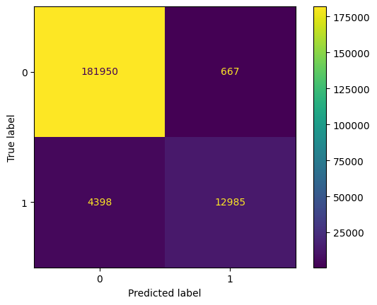
Here is the order of the fields from Sally's transaction details:
- distance_from_last_transaction
- ratio_to_median_price
- used_chip
- used_pin_number
- online_order
We are predicting whether a specific transaction (Sally's transaction) is fraudulent and determining the likelihood of fraud.
sally_transaction_details = [
    [0.3111400080477545,
    1.9459399775518593,
    1.0,
    0.0,
    0.0]
    ]

prediction = sess.run([output_name], {input_name: scaler.transform(sally_transaction_details).astype(np.float32)})

print("Is Sally's transaction predicted to be fraudulent? (true = YES, false = NO) ")
print(np.squeeze(prediction) > threshold)

print("How likely was Sally's transaction to be fraudulent? ")
print("{:.5f}".format(100 * np.squeeze(prediction)) + "%")
The model predicts that Sally's transaction is not fraudulent, with a fraud likelihood of only 0.01226% This suggests the transaction is considered safe based on the model's analysis.
Expected output:
Is Sally's transaction predicted to be fraudulent? (true = YES, false = NO)
False
How likely was Sally's transaction to be fraudulent?
0.01226%
Summary
This learning exercise provided a step-by-step process for developing and evaluating a fraud detection model using TensorFlow and ONNX on Red Hat’s OpenShift AI platform. Starting from the Jupyter notebook setup in the Red Hat Developer Sandbox, we configured a TensorFlow workbench and created a neural network tailored for detecting fraudulent transactions. We evaluated model performance with key metrics, then converted the model to ONNX format for efficient deployment. Finally, we demonstrated the model’s accuracy with a confusion matrix and conducted prediction tests to verify its fraud detection capabilities.
