Deep neural networks are achieving the incredible, pushing the boundaries of artificial intelligence in areas from medicine to language. But as these powerful AI systems become more integrated into our lives, a critical challenge looms: we often don’t understand how they arrive at their answers. They operate like inscrutable “black boxes,” making it hard to fully trust them.
The field of mechanistic interpretability strives to crack open these boxes. Our recent research paper, described in this post, offers a fresh perspective on this vital mission, introducing a new "combinatorial" way to potentially decode AI’s hidden logic. Understanding these systems isn’t just fascinating—it’s fundamental to building the safe, reliable AI of the future.
The current view: Looking at shapes in “activation space”
Much exciting research has tried to peek inside these black boxes by looking at the patterns of activity within the network. Imagine the network’s internal state as a point in a vast, high-dimensional space. (Think thousands or millions of dimensions!) Researchers track how this point moves as the AI processes information. Using clever techniques (like specialized tools called “sparse autoencoders”), scientists have discovered fascinating things:
Features: Specific concepts or patterns the AI seems to recognize (like “cat fur” or “happiness”).
Polysemanticity: Sometimes, a single internal component (a “neuron”) seems to represent multiple, unrelated features during different computations.
Superposition hypothesis: Features often aren’t neatly separated; they overlap, represented by combinations of neurons, like chords in music rather than single notes. Since there are many more combinations available than single neurons, the network can represent many more features than it has neurons.
These geometric approaches have been incredibly valuable. They tell us some of the features the network learns and roughly how they are represented. However, they do not explain the step-by-step calculations the network performs to combine these features and reach a conclusion. It’s like knowing the ingredients in a cake but not the recipe instructions.
A new angle: Thinking in combinations, not just geometry
Our recent paper proposes a different way to look inside the neural network: a combinatorial approach. Instead of focusing on the exact numerical values flowing through the network or their geometric positions, we focus more on the structure and relationships encoded in the network’s parameters (its learned “weights” and “biases”). Think of it as going from analyzing the voltage levels in a live circuit to reading the circuit’s wiring diagram itself.
To make this easier initially, we started by looking at how networks learn simple logic problems, using Boolean expressions (such as A ∧ B or C ∨ D, where ∧ is the logic AND and ∨ is the logical OR). This simplified setting helps us uncover fundamental computational mechanisms. Our goal is to build a theory explaining how neural networks compute—at least for these logic tasks—by showing that features and calculations are represented as specific combinatorial structures: patterns baked into the network’s learned settings. We specifically focus on patterns in the sign-based categorization of those settings (positive, negative, or zero).
Introducing the feature channel coding hypothesis
At the heart of our approach is an idea we call the feature channel coding hypothesis. It explains two key things:
How features are represented: Like the superposition hypothesis, we believe features aren’t usually represented by single neurons. Instead, each feature is represented by a specific set of neurons—its “code.” Think of it like a unique barcode for that feature within a layer of the network. If the codes for two different features don’t overlap much, the network can keep them relatively distinct. This aligns with the geometric idea (going further into the superposition hypothesis) of features being “almost orthogonal” (at right angles in that high-dimensional space).
How computation happens (the key difference): This is where our theory offers a new perspective. To compute a new feature (say, f) that depends on earlier features (say, x and y), the network essentially maps the codes for x and y onto the code for f. The actual calculation needed to compute f (e.g., if f = x ∧ y, the math might be something like “activate if x + y — 1 is positive”) is then performed individually by each neuron in f ’s code.
If the right combination of input features (x and y) are active, all the neurons making up f’s code will also become active, which means that feature f itself becomes active. The “code” for f acts like a dedicated computational channel, bringing together the necessary inputs for the computation of f. There might be some “noise” or interference if codes overlap, but if the overlap is small, the computation still works reliably.
Why is this exciting? If this hypothesis holds, we can potentially:
Decode the network’s logic: By finding these codes directly within the network’s learned parameters (weights and biases), we can reconstruct the “circuit diagram” of its computation.
Do it statically: We can understand the computation just by looking at the network’s final learned structure, without needing to run data through it constantly or train other AI models (like autoencoders) to interpret the first one. We can aim to understand the how, the low-level mechanics, not just the what and where of feature dependencies.
What we found (in a nutshell)
Our paper presents evidence supporting this combinatorial view:
It happens! We showed that feature channel coding naturally emerges when training standard neural networks (specifically, Multi-Layer Perceptrons or MLPs) on various logic problems. We even saw it arise in a simple task mimicking computer vision. Crucially, for some examples, we successfully extracted the complete set of codes and the exact computations directly from the network’s learned parameters.
It’s not random and it explains polysemanticity, superposition, and scaling laws. We measured how often these code structures appear and found it’s far more frequent than chance. This approach also offers a potential explanation for why AI models sometimes break down as problems get more complex: there might be a fundamental limit to how many unique “codes” can be packed into the network, even with superposition, without them interfering too much. We also watched these codes gradually form during the training process, which could help us understand how different training techniques affect learning.
A simple example: How networks naturally learn feature channel coding
Let us take one example from the paper to see how feature channel coding naturally emerges. We conducted a simple experiment using a foundational neural network structure called a multilayer perceptron (MLP).
Think of an MLP as an assembly line for information. It has distinct stages, called layers. Our MLP had three main stages:
- Input layer: This first stage simply received the raw data—in our case, 16 different input variables.
- Hidden layer: The input data was then passed to a processing layer with 16 neurons. This is where intermediate calculations happen.
- Output layer: Finally, the results from the hidden layer were sent to a single neuron in the output layer, which produced the final result of the computation.
These layers were fully connected, meaning every unit in one layer sent its output to every unit in the next layer.
Now, how does the network actually learn? Each of these connections has an adjustable "weight," like a volume knob controlling the strength of the signal passing through. Additionally, each neuron in the hidden layer has a "bias," another adjustable knob that acts like a minimum threshold the incoming signals must overcome for the neuron to activate.
"Training" the network is the process of automatically tuning all these parameters (the "weight" and "bias" knobs) so that the network consistently produces the correct output for a given input. In our case, we had the network learn to solve the following randomly generated logic problem.
f(x0,…,x15) =(x3∧x11)∨(x9∧x13)∨(x2∧x6)∨(x0∧x4)∨(x5∧x12)∨(x7∧x15)∨(x8∧x10)∨(x1∧x14)
We provided the network with 30,000 random binary inputs, each representing different combinations of True (1) or False (0) values. Each input randomly contained between two and six variables set to True. The network was trained using standard techniques (binary cross-entropy loss and the Adam optimizer) for 2,000 iterations (epochs).
We want to look "under the hood" at the connections our neural network learned, searching for direct evidence of "feature codes" in the connection strengths (weights). To do so, we visualized the learned weights and biases of our neural network using heat maps like in the following figures.
Figure 1 shows the Layer 1 matrix W1 (all the Layer 1 weights), its Layer 1 bias, and the Layer 2 matrix W2 (a single neuron with weights matching each of the neurons in Layer 1, so it is just a vector). The colors correspond to the sign and magnitude of the weights: the bluer they are the more positive, the redder the more negative.
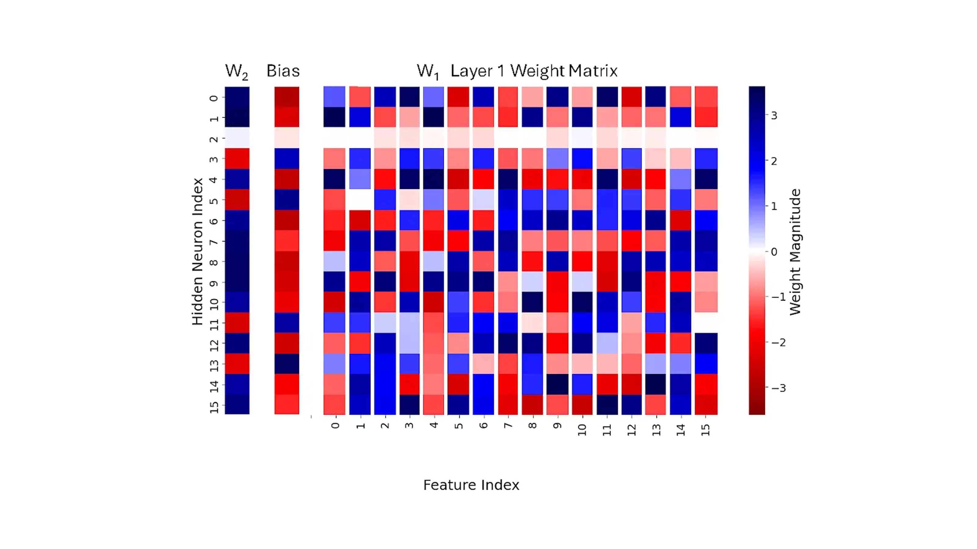
First, let's focus on W1. The weight matrix in the figure is in its raw form without alteration. Its columns correspond to input features, the input values of the variables, and its rows correspond to the neurons in the hidden layer. The value of a matrix entry is the weight of the connection between the corresponding input neuron for its column and the hidden neuron for its row. The matrix W1 does not seem to reveal much, other than the fact that neuron 2 does not really participate in the computation.
Next, we look at the same information slightly differently in Figure 2.
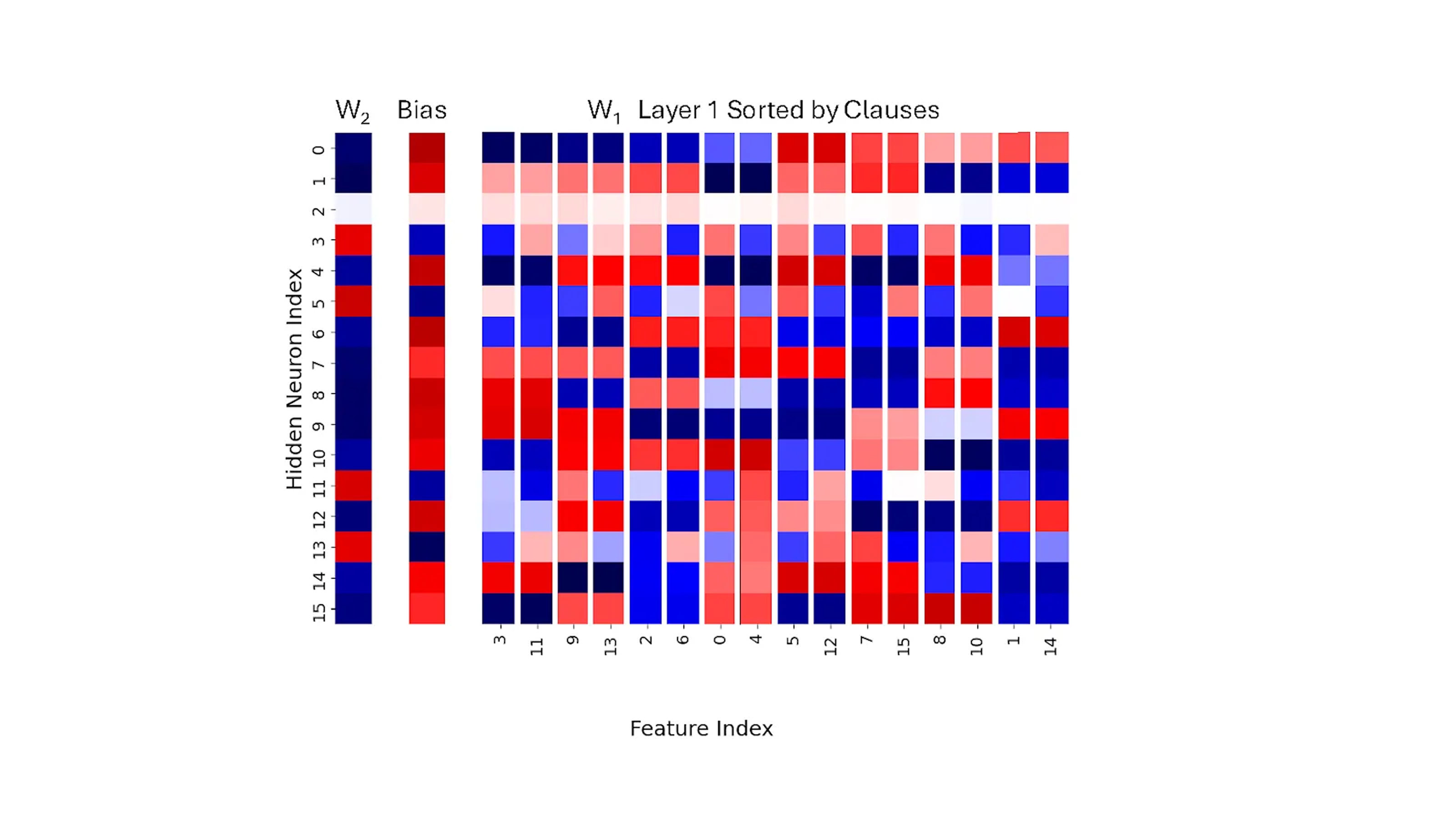
In this second version of the heat map, we sorted the columns of W1 by the features (variables) so that the pairs that are joined by an AND, in the formula the network is trained on, are next to each other. So, for example, columns 3 and 11 are next to each other because (x3 ∧ x11) is an AND clause in the formula. This image starts to reveal that there is something interesting going on with these pairs: in many positions, but not all, adjacent columns have the same values.
Figure 3 shows yet another view into the same information.
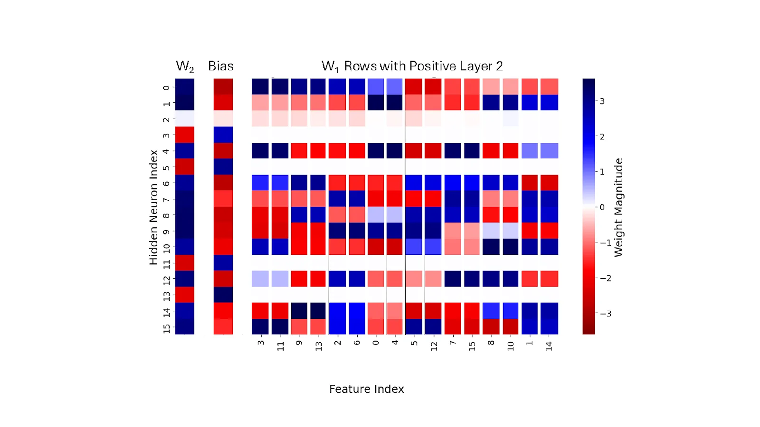
In this third version, columns of W1 are again sorted by the features, but now we only include the rows (neurons) of the weight matrix W1 that correspond to positive values in W2, the Layer 2 weights (we will see below that these are the rows that promote a True output). This image is striking: in each and every row, the columns corresponding to an AND feature pair seem to be virtually identical. Moreover, if we look at the positive, blue colored weights, we see an emerging pattern.
Looking across all pairs of input features (variables), every pair that appears in the same AND feature is in fact brought together into a feature channel code. The set of neurons in that code allows the AND feature’s computation to propagate to the next layer.
For example, in the underlying computation, input features 3 and 11 are used to compute the output feature (x3 ∧ x11). Thus, they are mapped to the same feature channel code, which consists of positive (blue) weights on the set of neurons {0,4,6,10,12,15}. Feature (x9 ∧ x13) is represented by the code {0,6,8,14}, and feature (x5 ∧ x12) by the code {6,8,9,10,15}.
But how is the code used to compute a feature? Let’s consider the feature (x3 ∧ x11). The network computes this using the neurons of the code for inputs x3 and x11: the neurons in the set {0,4,6,10,12,15}. To see how, imagine first that you had a single neuron to compute (x3 ∧ x11). Mathematically, (x3 ∧ x11) = ReLU(x3 + x11–1), where ReLU stands for Rectified Linear Unit, a widely used activation function in deep learning, defined as ReLU(x) = max(0, x). So if the inputs to both x3 and x11 are a 1 value, the neuron will return a 1, and if either (or both) is a 0, it will return a 0, and so the neuron is exactly computing (x3 ∧ x11).
However, the neural network does not compute using exact Boolean logic, but rather using soft Boolean logic, where the -1 is replaced by a -b for some real value b. And indeed, as if by magic, we see in the heat map that for every single row with a positive Layer 2 weight, the network learned a bias that is significantly negative, representing the −b.
The key to feature channel coding is that the weights in the two columns are essentially the same (columns 3 and 11 are identical), and so the set of rows (neurons) where positive values appear in those columns can be used to compute the AND of those two inputs using this exact formula. When x3 and x11 are both 1s and all other inputs are 0s, then in the neural network computation with this input, all of the coding neurons {0,4,6,10,12,15} use columns 3 and 11 to produce a positive sum after subtracting the bias and applying a ReLU, while all other neurons will produce 0. This activates exactly those neurons in the code for (x3 ∧ x11). The code consisting of those neurons serves as a “computational channel” for computing (x3 ∧ x11), detected by the Layer 2 neuron since each of these positive values is multiplied by a positive Layer 2 weight. Consequently, the result from the network will be True.
Polysemanticity and superposition in action
The network above demonstrated polysemanticity—neurons that respond to multiple unrelated clauses. For example, neuron 4 was activated by four different logical pairs: (x3 ∧ x11), (x0 ∧ x4), (x7 ∧ x15), and (x1 ∧ x14). The result of neuron 4 will be similar when the input consists of 1s for only variables x3 and x11 (a True instance) to what it is when the input consists of 1s for only variables x3 and x4 (a False instance).
However, the other rows of the code for (x3 ∧ x11) make up for this: only neurons 0 and 4 activate when the input is 1s for variables x3 and x4. Feature channel coding ensures that the correct logical signals are detectable by encoding each logical pair across multiple neurons. Thus, even though overlap occur, correct signals are much larger than false ones. For example, when the input has 1s for only variables x3 and x11, six neurons activate, but for inputs with 1s for only x3 and x4, only two neurons activate.
The superposition hypothesis suggests that features are represented as almost-orthogonal directions in the vector space of neuron outputs, but does not explain how they are computed. Feature channel coding proposes the first concrete explanation of how computation of features in superposition might actually be conducted.
Negative rows
Since some positive signal does get through even with the False instance, we see that the negative rows do play a role in the computation. With this as motivation, let us get back to the separation of the weight matrix into the rows that have positive Layer 2 weights and those that have negative Layer 2 weights. Figure 4 shows the same sorting of the columns as before, but this time just the negative W2 weight rows.
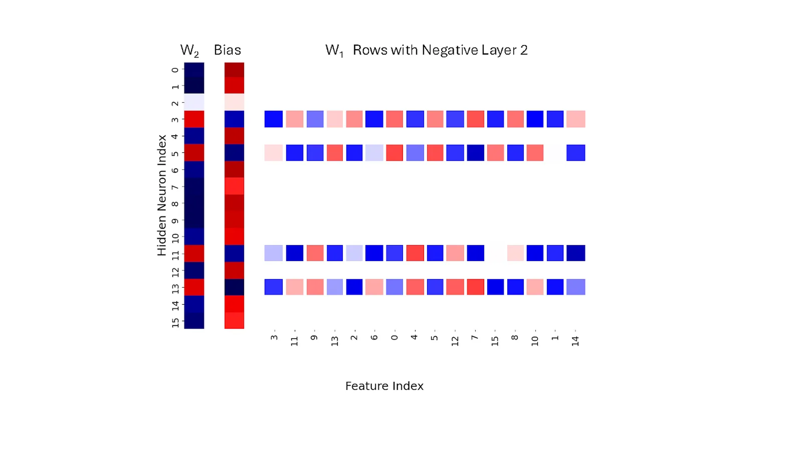
Let’s look at neuron 3. If inputs x3 and x4 are ‘on’, neuron 3 sends a strong ‘off’ signal to the output. Why? Although neuron 3 activates positively (due to positive settings for x3 and x4, as well as a positive bias), its connection to the output (in W2) is negative, flipping this signal to strongly negative. This overrides weaker ‘on’ signals from other neurons (0 and 4). However, if x3 and x11 are both ‘on’, neuron 3’s ‘off’ signal is much weaker. This is because the weights for x3 and x11 have opposite signs, preventing strong activation. This behavior highlights a key learning outcome: the network prefers inputs in the same clause to have opposing Layer 1 weights within these negative rows.
More generally, the sign of the Layer 2 weights in W2 defines whether a row of the W1 matrix contributes to the final result as a positive or a negative value. Essentially, the positive W2 weights correspond to features in Layer 1 that we call positive witnesses: they provide evidence that the input is a 1 (True) instance and provide a strong positive signal to support that. Negative W2 weights are negative witnesses and provide a negative signal due to evidence that the input is a 0 (False) instance.
Scaling laws through the lens of feature channel coding
A scaling law in neural networks describes how model performance systematically improves as factors like model size, dataset size, or computational resources increase. These laws help researchers forecast performance gains when scaling up neural network architectures.
We next show that the properties of feature channel coding explain the shape of a specific scaling law. This is interesting, because while scaling laws are very well studied, they do not typically come with an explanation of why they occur and what the underlying constraint is that increasing resources help alleviate. Unlike most scaling law studies, our focus on Boolean formulas allowed us to control the number of features explicitly, facilitating a more precise analysis.
We trained networks like the one described above to learn a formula consisting of an OR of 64 clauses, where each clause is an AND of 4 disjoint variables. Thus, the number of output features is fixed at 64, and we also kept the number of input features fixed at 32. We study the impact of increasing the size of the hidden layer from 4 to 128 neurons, with a specific focus on the coding patterns that emerge. We saw that in the positive rows (positive witnesses) it uses a coding pattern of 4 positive weights per row for each clause, since the clauses now consist of 4 distinct variables (instead of the 2 positive weights and 2 variables per clause we saw for the example above). We call this coding pattern 4P, i.e., 4 positive weights.
In the negative rows, the most prevalent pattern was 3 negative weights and one positive one (we call this 3N1P). We want to measure the average size of the resulting codes: on average, how many rows does this coding pattern appear in for each clause? We plot the change in training and test error and the frequency of 4P codes in positive rows (blue) and 3N1P codes in negative rows (green) as we increase the size of the hidden layer j from left to right. We see that the decrease in error is closely related to the increase in code frequency.
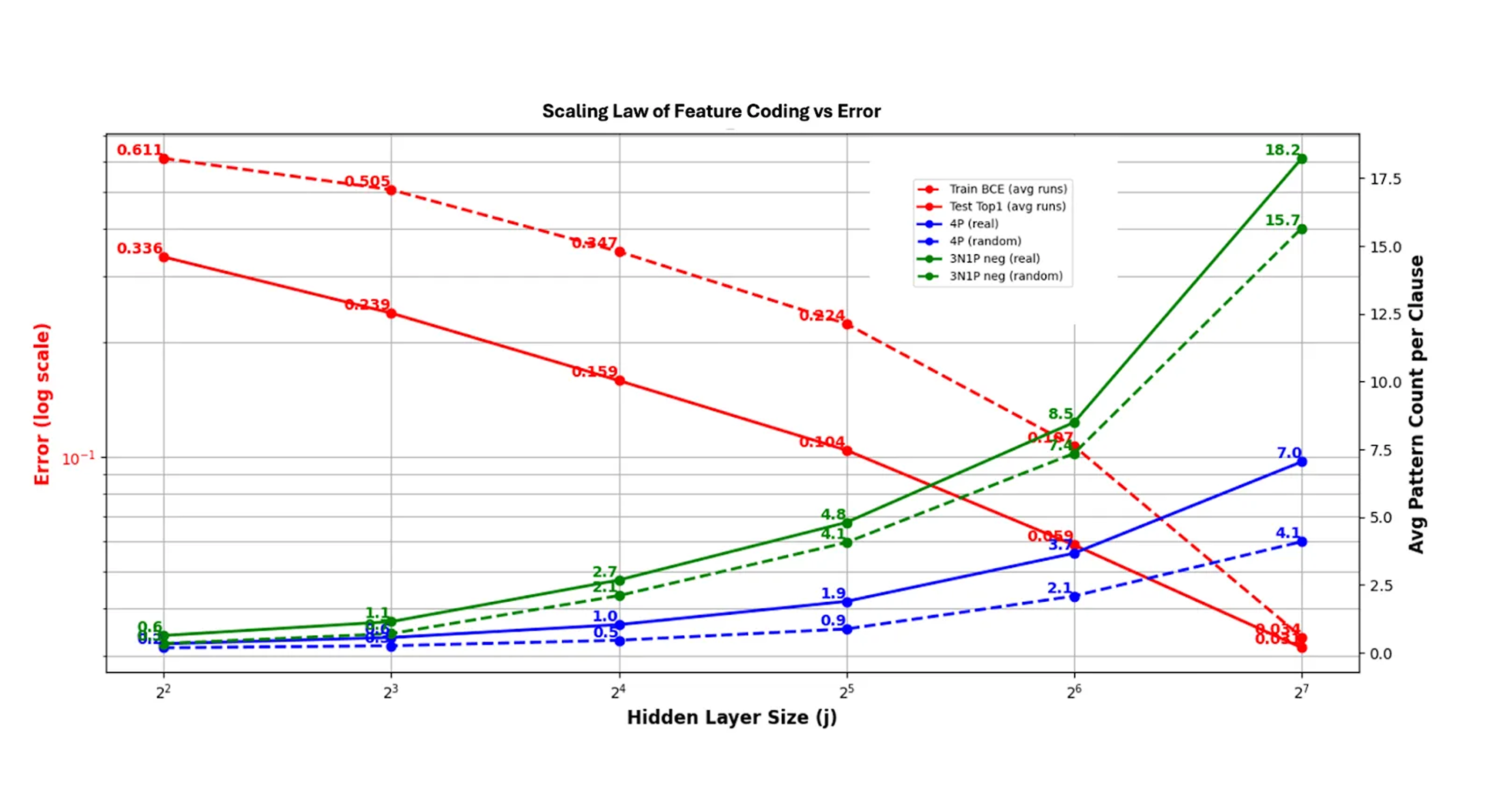
We believe that this relationship is due to the capacity of the network to perform feature channel coding: there are a limited number of entries in the weight matrix W1, and so there is a limit to how many of the 4P patterns for coding can fit into that matrix. We found that the network essentially achieves that limit, but is not able to go beyond that. This provides an easily explainable scaling law: the network’s size implies a capacity to code feature channels, with smaller networks being more limited in their coding ability, which explains the higher error rate.
We also point out that in all cases, both patterns appear more frequently than random (solid lines versus dashed lines). The 4P positive coding is potentially more dominant as a code, hinted at by its relative ratio to the random distribution. As networks grow, the ratio of 4P to 4P-random starts around 2, and decreases, but still is at almost 1.7x with 128 hidden neurons, while the ratio of 3N1P to 3N1P-random is at 1.16 with 128 hidden neurons. One could envision building on this to use the ratios of codes in smaller models to derive scaling predictions for larger models, a new more refined approach to scaling that merits further research.
Why this matters
Our experimental work above clearly shows neural networks naturally adopt a combinatorial coding structure, at least when learning to compute Boolean formulae. They spontaneously learn to represent logical operations as specific neuron groups, providing a clear, interpretable “wiring diagram.” It’s a promising step toward understanding how neural networks truly compute and reason, moving beyond geometry and activations to decode their actual logic circuits.
Looking ahead
This combinatorial perspective doesn’t replace the geometric view; they are complementary ways of understanding AI. However, we believe looking at the network’s structure through this “coding” lens offers unique insights into the mechanics of computation. While our examples are currently small, we hope this approach can be scaled up. Understanding the precise “circuits” inside AI could lead to breakthroughs in debugging, ensuring safety, improving efficiency, and truly grasping how these powerful systems learn and reason. It’s a step towards turning the black box into something more understandable, one code at a time.
Last updated: April 24, 2025